How to Flexibly Control Entropy in LLM Reinforcement Learning

This article introduces our recent research on RLVR training dynamics. Starting from a theoretical perspective of Gradient-Preserving Clipping, we propose a flexible entropy regulation mechanism. Based on the entropy-increasing and entropy-decreasing regulation mechanisms, we experiment with three entropy control strategies: increase-then-decrease, decrease-increase-decrease, and oscillatory decay. Through experiments, we demonstrate that these strategies effectively mitigate the policy entropy collapse problem in GRPO training.

This is the English translated version.

Paper: Flexible Entropy Control in RLVR with Gradient-Preserving Perspective

Paper link: http://arxiv.org/abs/2602.09782

1. Background: When LLMs Become “Prematurely Confident”

In recent years, large language models represented by DeepSeek-R1 have achieved remarkable progress in mathematical reasoning, code generation, and other tasks through RLVR. As a representative RLVR algorithm, GRPO has been widely adopted due to its simplicity and efficiency — it requires no separate Critic network. However, a pervasive phenomenon troubles researchers: as training progresses, the policy entropy rapidly decays to near zero — this is entropy collapse.

What Is Policy Entropy Collapse?

Policy entropy measures the “uncertainty” or “diversity” of model outputs. High entropy means the model explores diverse solution paths, while low entropy means the model becomes “overconfident,” tending to repeat a few fixed patterns.

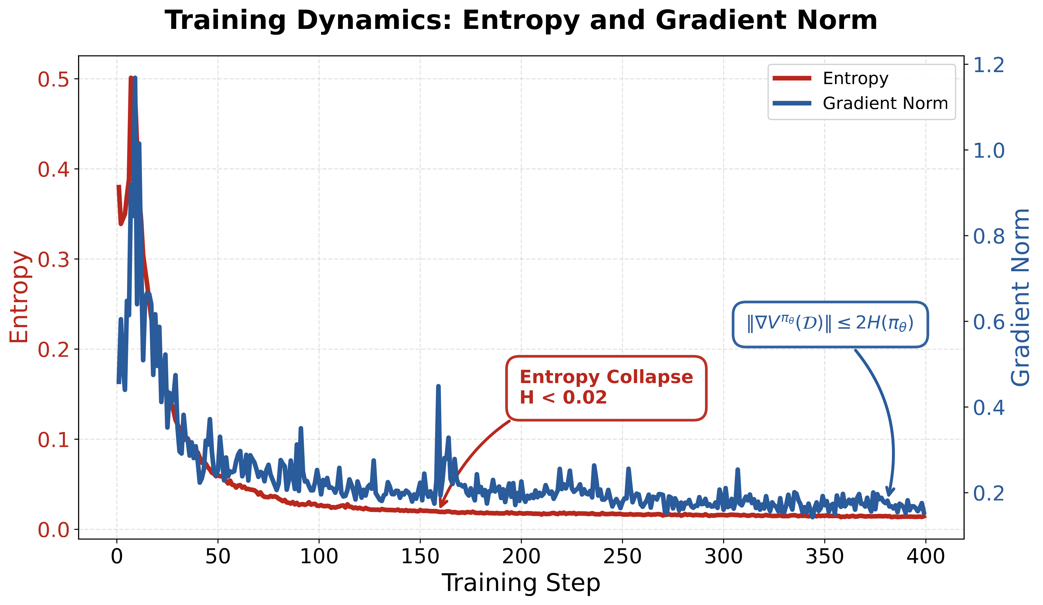
Figure 1: During GRPO training, policy entropy rapidly decays (entropy collapse), while gradient norms are bounded by the entropy upper bound

GRPO training often exhibits rapid entropy decay, i.e., entropy collapse. Entropy collapse brings two serious consequences:

1. Premature convergence: The model locks onto a few “seemingly effective” solution strategies early in training, loses exploration capability, and gets trapped in local optima
2. Gradient vanishing: Theoretical analysis by Shen et al. shows that policy gradient norms are bounded by entropy — entropy collapse directly leads to weak gradients in subsequent training, making it difficult for the model to continue improving

---

2. Root Cause: The Double-Edged Sword of Gradient Clipping

To understand entropy collapse, we need to return to the core mechanism of RLVR — PPO-Clip’s gradient clipping.

PPO-Clip Review

PPO (Proximal Policy Optimization) stabilizes training by limiting the deviation between new and old policies:

\[r_t(\theta) = \frac{\pi_\theta(a_t|s_t)}{\pi_{\text{old}}(a_t|s_t)}\]

where $r_t(\theta)$ is the importance sampling ratio. The PPO-Clip objective function is:

\[L^{C}(\theta) = \hat{\mathbb{E}}_t \left[ \min \left( r_t(\theta)\hat{A}_t, \text{clip}(r_t(\theta), 1-\epsilon, 1+\epsilon)\hat{A}_t \right) \right]\]

By clipping $r_t(\theta)$ within the interval $[1-\epsilon, 1+\epsilon]$, PPO ensures that policy updates are not overly aggressive.

The Subtle Relationship Between Clipping Thresholds and Entropy

Existing research (e.g., DAPO) has found that overly strict clipping thresholds suppress the exploration of low-probability tokens, leading to continuous entropy decline. DAPO’s proposed Clip-Higher strategy alleviates this by raising the upper bound threshold $\epsilon_{high}$.

However, what exactly is the relationship between gradient clipping and entropy control? Can we accurately and flexibly control entropy increase and decrease through gradient clipping? And how should we effectively control entropy during training? Our core contributions answer these three questions.

3. Theoretical Analysis: Four Entropy-Sensitive Regions

One of our contributions is theoretically characterizing precisely which regions in the importance sampling ratio space promote entropy growth and which lead to entropy decline. We found that our discussion coincides with recent work by the Tongyi team, On the Entropy Dynamics in Reinforcement Fine-Tuning of Large Language Models. Their Zhihu introduction RL训练中的 Entropy Dynamics also provides discussion of this theory and other related works.

Core Derivation

For the single-step update surrogate objective:

\[L(\theta) = \frac{\pi_\theta(a|s)}{\pi_{\text{old}}(a|s)} \hat{A}\]

We compute the inner product of the objective function gradient and the global entropy gradient:

\[\langle \nabla_z L, \nabla_z H \rangle \propto -\hat{A} \left[ p_a(\ln p_a + H) - \sum_{x \in V} p_x^2 (\ln p_x + H) \right]\]

The two terms are the token-specific term and the global baseline term, respectively. The sign of this inner product is primarily determined by the token-specific term relative to the baseline. Focusing on the token-specific component, we obtain:

\[\langle \nabla_z L, \nabla_z H \rangle \propto -\hat{A} \left[ p_a(\ln p_a + H)\right]\]

This yields a key insight: the direction of entropy change depends on the relative relationship between a token’s “surprisal” and the current entropy.

Four Entropy-Sensitive Regions

Based on our theoretical analysis, we identify four key regions:

Region	Condition	Advantage $A$	Entropy Change
E1	$-\ln \pi(a|s) < H$ (low surprisal / high probability)	$A > 0$	Decrease
E2	$-\ln \pi(a|s) > H$ (high surprisal / low probability)	$A > 0$	Increase
E3	$-\ln \pi(a|s) < H$ (low surprisal / high probability)	$A < 0$	Increase
E4	$-\ln \pi(a|s) > H$ (high surprisal / low probability)	$A < 0$	Decrease

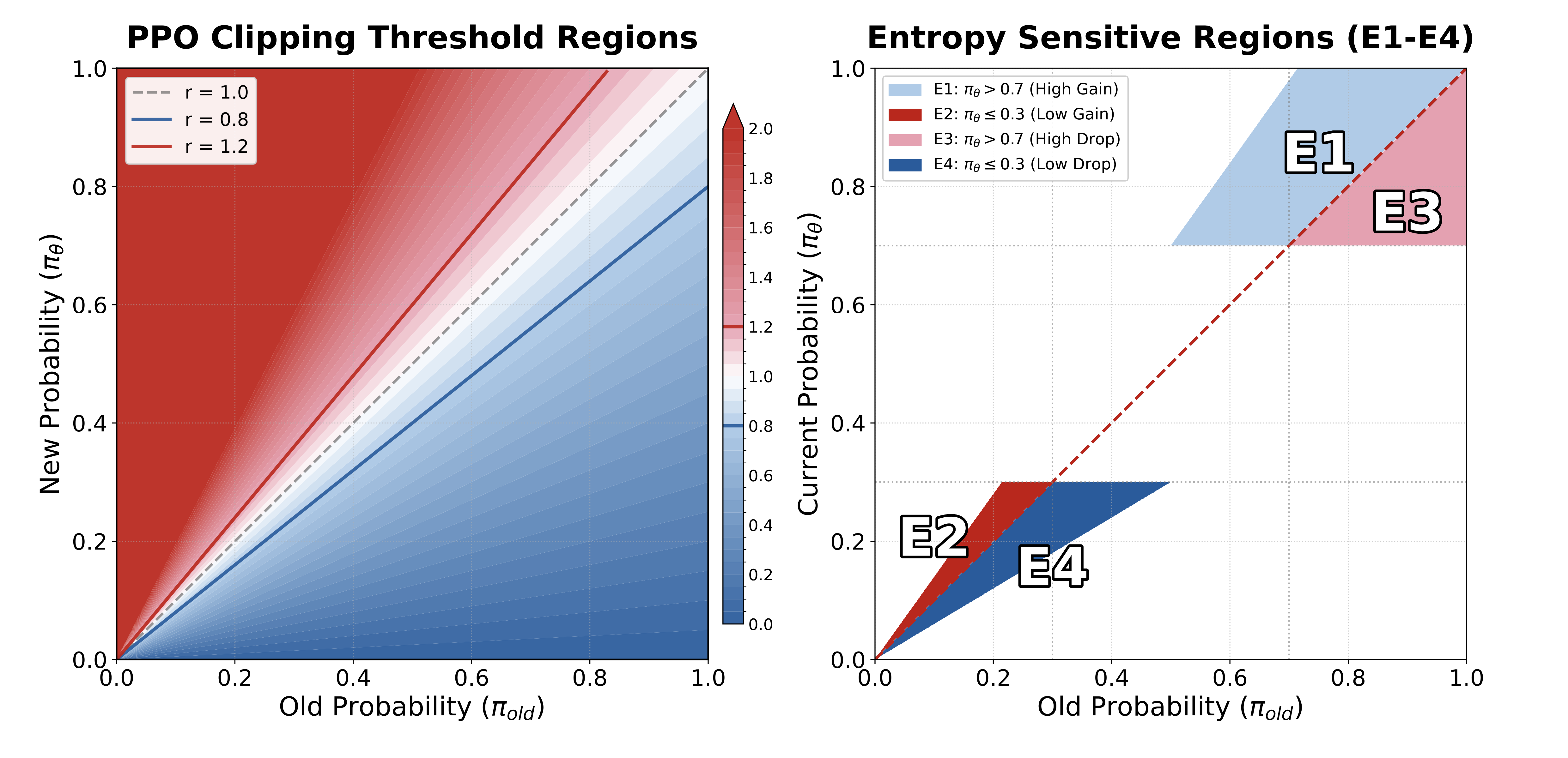
Figure 2: PPO clip schematic and the four regions

Intuitive understanding:

• E1/E4: Reinforcing “expected” tokens → sharper distribution → entropy decrease
• E2/E3: Reinforcing “surprising” tokens → flatter distribution → entropy increase

We verified this theory through controlled experiments: applying gradient clipping only to specific regions, we observed entropy dynamics fully consistent with theoretical predictions.

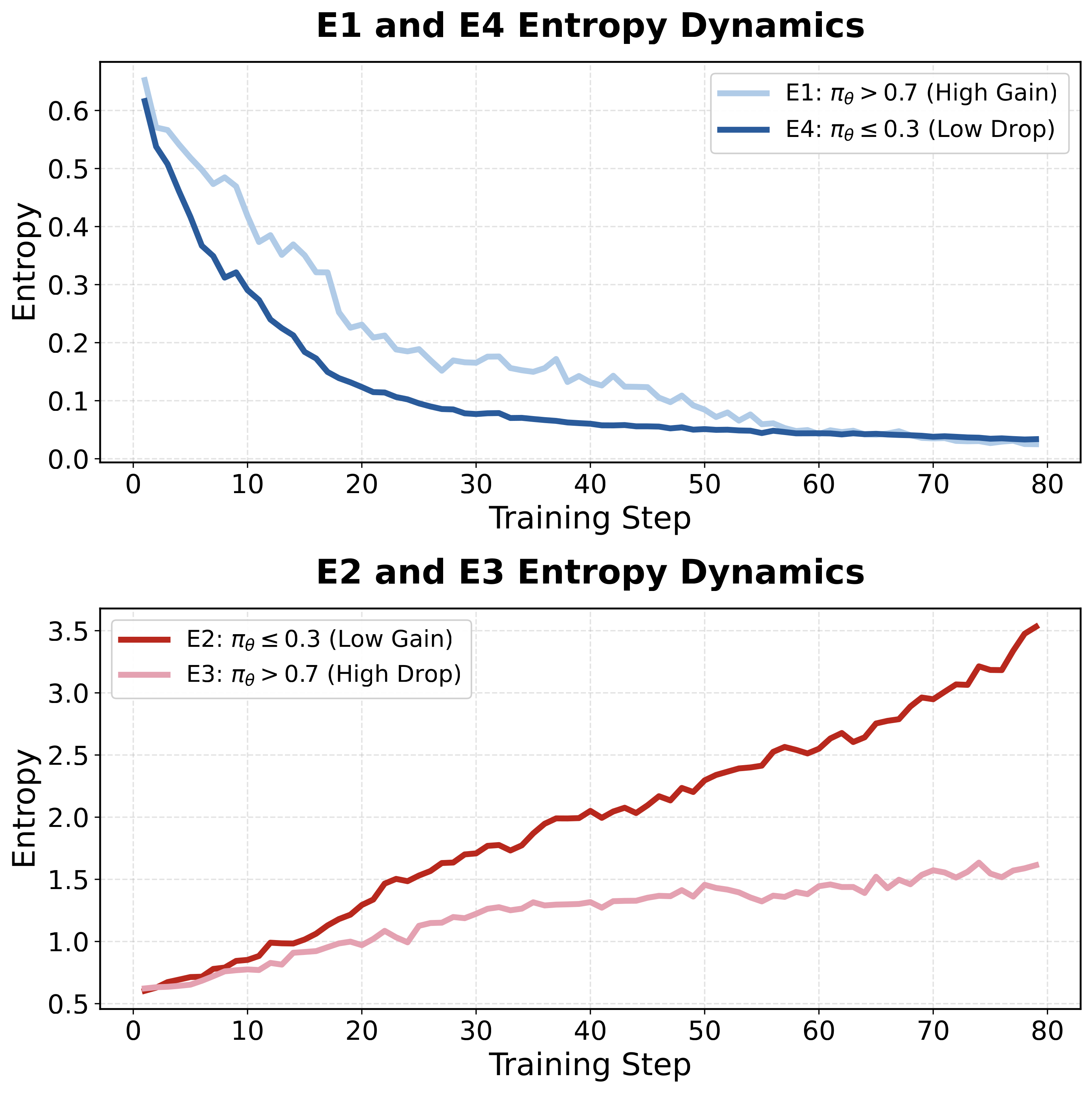
Figure 3: Entropy dynamics for the four regions. E1/E4 lead to entropy decrease, E2/E3 lead to entropy increase

---

4. Entropy Regulation Mechanism: Dynamic Clipping Thresholds

Based on the above theoretical insights, we design a dynamic clipping threshold mechanism that precisely controls entropy through nonlinear modulation of specific ratio regions.

4.1 Dynamic Upper Clipping Threshold (Controlling Entropy Increase)

When $A > 0$, the upper threshold primarily affects the E1 (high probability) and E2 (low probability) regions.

A fixed high threshold (e.g., DAPO’s clip-higher), while promoting exploration in the E2 region, simultaneously introduces over-optimization in the E1 region, leading to entropy decrease. To avoid this, we design the upper threshold $\epsilon$ as a function of the current probability:

\[\epsilon(\pi_\theta) := f(\pi_\theta(a_t|s_t))\]

where $f$ is negatively correlated with $\pi_\theta$:

• Low-probability tokens: Relax the threshold to promote exploration (enhance E2)
• High-probability tokens: Tighten the threshold to prevent over-optimization (suppress E1)

Using a linear negative correlation $\epsilon(\pi_\theta) = \alpha \cdot \pi_\theta + \beta$, we obtain the dynamic constraint:

\[\pi_\theta(a_t|s_t) \le \frac{1+\beta}{1-\alpha \cdot \pi_{\theta_{\text{old}}}(a_t|s_t)} \cdot \pi_{\theta_{\text{old}}}(a_t|s_t)\]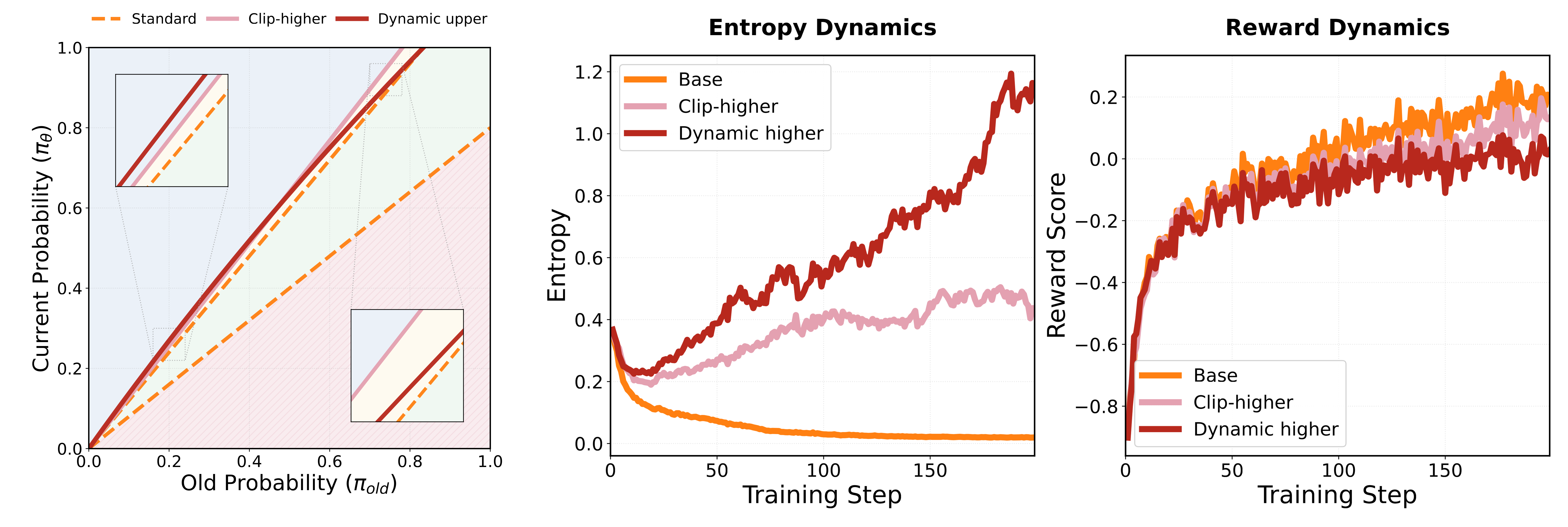

Figure 4: Dynamic upper clipping threshold. The threshold in the low-probability region is higher than the baseline, while the threshold in the high-probability region is lower than the baseline

4.2 Dynamic Lower Clipping Threshold (Controlling Entropy Decrease)

When $A < 0$, the situation is more subtle. Negative advantage signals have an instability problem: due to the normalization property of Softmax, penalizing one token indirectly increases the probabilities of all other tokens. For high-probability negative samples, a fixed high $\epsilon_{low}$ allows excessive updates, causing drastic distribution shifts. For low-probability negative samples, further reducing their probability helps eliminate suboptimal regions with limited impact on the overall distribution.

Therefore, we adopt the opposite dynamic strategy:

• High-probability tokens: Tighten the threshold to maintain stability (suppress excessive entropy increase from E3)
• Low-probability tokens: Relax the threshold to strengthen elimination (enhance the entropy-decreasing effect of E4)

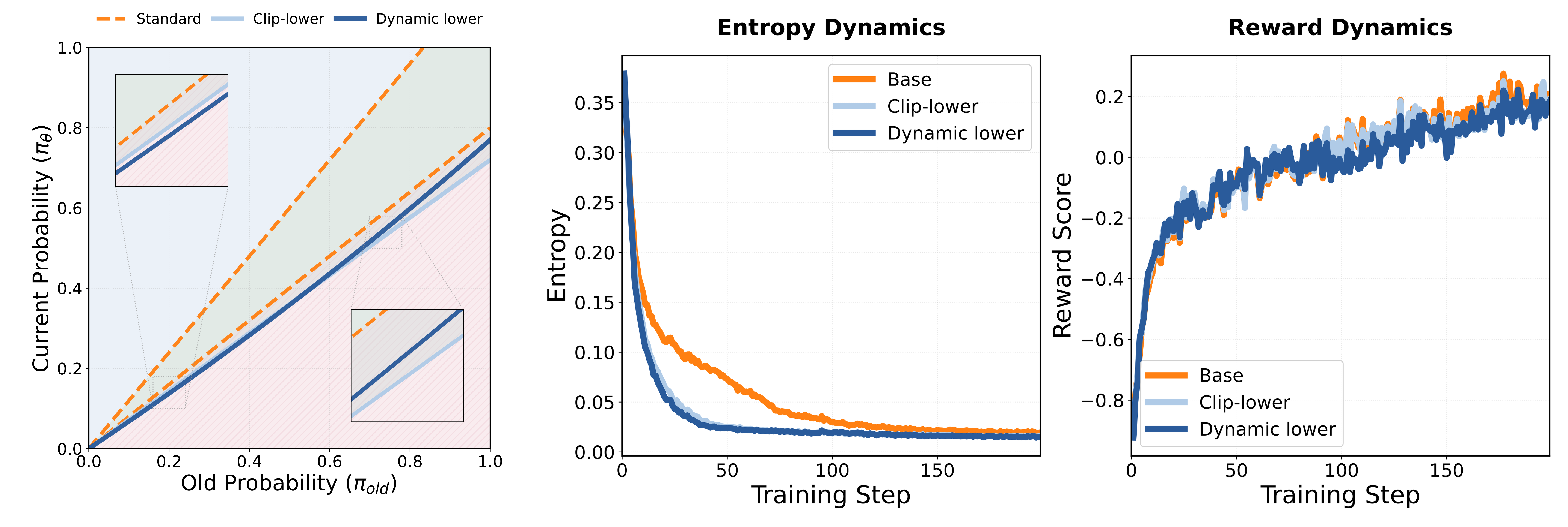
Figure 5: Dynamic lower clipping threshold (left) and its experimental effect (right). The threshold in the low-probability region is higher than the baseline, while the threshold in the high-probability region is lower — effectively promoting entropy decrease

---

5. Entropy Control Strategies: Balancing Exploration and Convergence

With the dynamic clipping mechanism, we can design flexible entropy control strategies. The core idea is: maintain high entropy early in training to promote exploration, then gradually reduce entropy later to achieve convergence.

We generalize the PPO clipping objective to a time-dependent form:

\[L^{CLIP}_k(\theta) = \hat{\mathbb{E}} \left[ \frac{1}{G} \sum_{t=1}^G \min \left( r_t(\theta) A_t, \text{clip}\left(r_t(\theta), 1-\mathcal{E}^-_k(p_t), 1+\mathcal{E}^+_k(p_t)\right) A_t \right) \right]\]

where $\mathcal{E}^+_k$ and $\mathcal{E}^-_k$ are threshold functions that dynamically change with training step $k$.

Strategy 1: Increase-then-Decrease (ID)

Using the midpoint of total training steps $T$ as the boundary, training is divided into two phases:

\[\mathcal{E}^+_{k-ID}(p), \mathcal{E}^-_{k-ID}(p) = \begin{cases} \lambda_k \cdot \mathcal{H}(p) + (1-\lambda_k) \cdot \epsilon_{std}, \quad \epsilon_{std} & 0 \le k \le \frac{T}{2} \\ \epsilon_{std},\quad (1+\lambda_k)\cdot \mathcal{M}(p)-\lambda_k\cdot \epsilon_{std} & \frac{T}{2} < k \le T \end{cases}\]

where $\lambda(k) = 1 - \frac{2k}{T}$, $\mathcal{H}(p)$ is the dynamic upper bound function, and $\mathcal{M}(p)$ is the dynamic lower bound function.

• Phase 1: Use the dynamic upper bound to promote entropy growth; the lower bound stays at standard value
• Phase 2: The upper bound returns to standard value; use the dynamic lower bound to promote entropy decrease

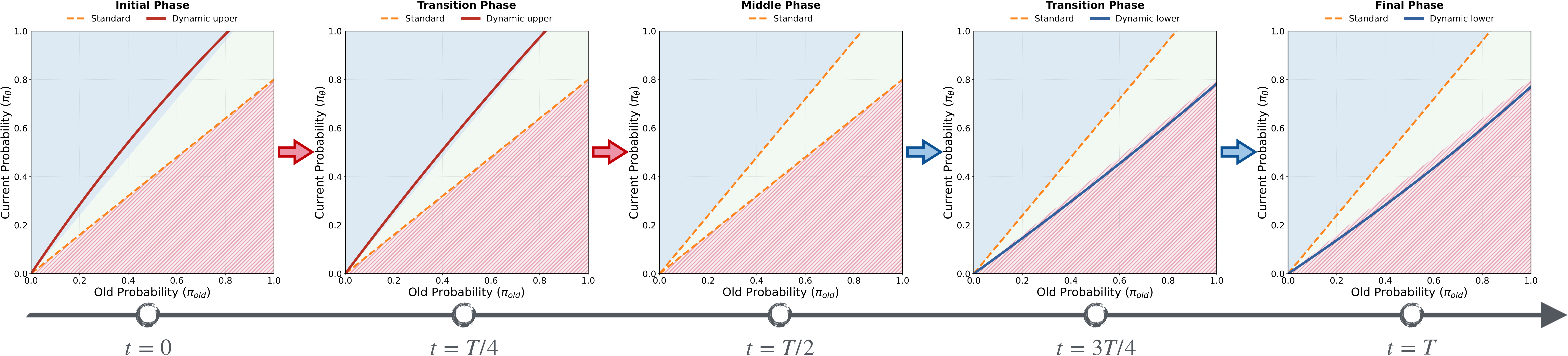
Figure 6: Two-phase entropy control schematic for the ID strategy

Strategy 2: Decrease-Increase-Decrease (DID)

The DID strategy allows entropy to first decrease in the first phase, then uses gradient clipping to control entropy recovery before entropy collapse, and finally converges in the second phase:

\[\mathcal{E}^+_{k-DID}(p), \mathcal{E}^-_{k-DID}(p) = \begin{cases} \lambda_k \cdot \epsilon_{std} + (1-\lambda_k) \cdot \mathcal{H}(p), \quad \epsilon_{std} & 0 \le k \le \frac{T}{2} \\ \mathcal{H}(p),\quad (1+\lambda_k)\cdot \mathcal{M}(p)-\lambda_k\cdot \epsilon_{std} & \frac{T}{2} < k \le T \end{cases}\]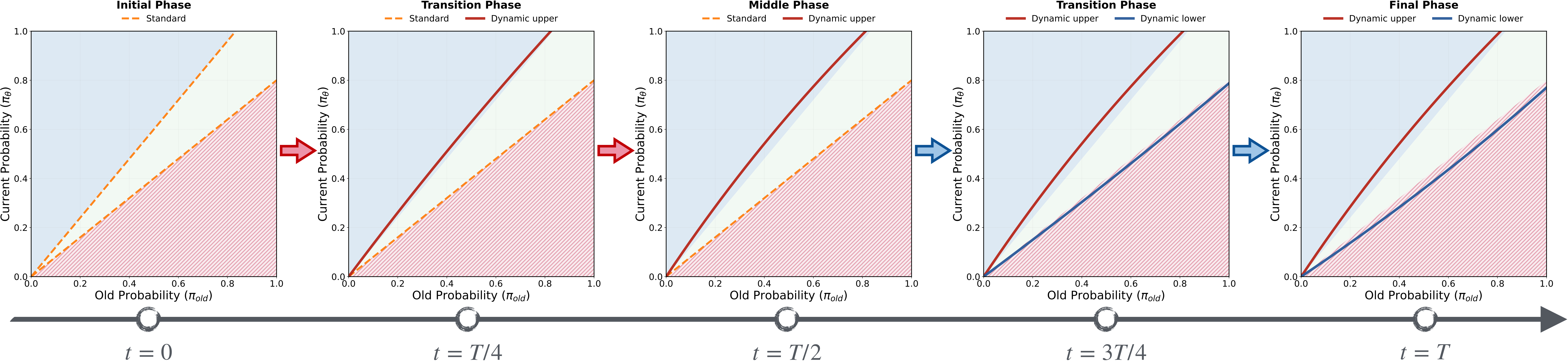

Figure 7: Three-phase entropy control schematic for the DID strategy

Strategy 3: Oscillatory Decay (OD)

Both ID and DID divide the training process into discrete phases. The OD strategy lets the model autonomously perform oscillatory decay throughout the entire training process:

Define the time-varying entropy thresholds:

\[\begin{aligned} \tau_{low} &= H_{min} \\ \tau_{high}(t) &= H_{min} + (H_{init} - H_{min}) \cdot \left(1 - \frac{t}{T}\right) \end{aligned}\]

where $H_{min} = 0.2 H_{init}$ is the target entropy lower bound.

Introduce a discrete state variable $s_k \in {0, 1}$ (1 for entropy-increasing mode, 0 for entropy-decreasing mode), with state transitions controlled by hysteresis logic:

\[s_k = \begin{cases} 1 & \text{if } H(\pi_t) \le \tau_{low} \quad (\text{trigger boost}) \\ 0 & \text{if } H(\pi_t) > \tau_{high}(k) \quad (\text{trigger suppression}) \end{cases}\]

Dynamically select clipping thresholds based on the current state:

\[\mathcal{E}^+_k(p), \mathcal{E}^-_k(p) = \begin{cases} \mathcal{H}(p), \quad \epsilon_{std} & \text{if } s_k = 1 \\ \epsilon_{std}, \quad \mathcal{M}(p) & \text{if } s_k = 0 \end{cases}\]

---

6. Experimental Results

We conducted comprehensive experiments on Qwen2.5-Math-7B and Qwen2.5-7B using the DAPO-MATH dataset, evaluating on AIME24, AIME25, AMC, MATH-500, GSM8K, Olympiad, and other benchmarks.

All three of our strategies outperform GRPO, Clip-Higher, and other baseline methods across multiple benchmarks. The ID strategy achieves the best performance on AIME24, AMC, MATH-500, GSM8K, and Olympiad. Detailed experimental results can be found in the paper.

Entropy and Reward Curve Analysis

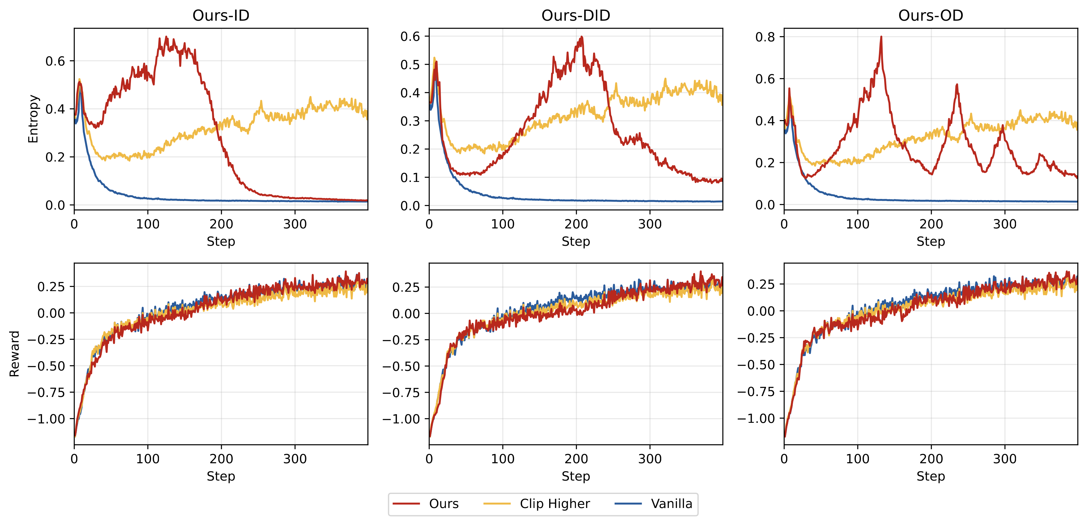
Figure 8: Training dynamics of each method on Qwen2.5-Math-7B

From the training curves, we observe:

1. Effective entropy regulation: All three strategies achieve the expected entropy change patterns
2. Later-stage performance superiority: Although early rewards are lower, our methods significantly surpass baselines in later stages

Exploration Capability Evaluation

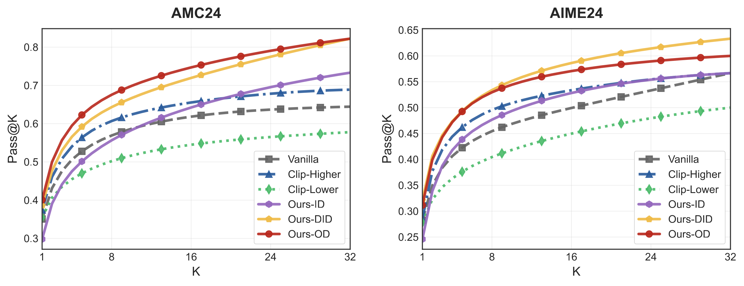
Figure 9: Pass@K performance of each method at mid-training (step 120)

We use the Pass@K metric to evaluate the model’s exploration capability at step 120, when model entropy is higher. Results show that while all methods perform similarly on Pass@1, with increased sampling, our methods demonstrate significantly better Pass@K performance, indicating that the model retains richer solution strategies.

Phase Ratio Analysis

For the ID and DID strategies, we analyze the impact of different phase ratios:

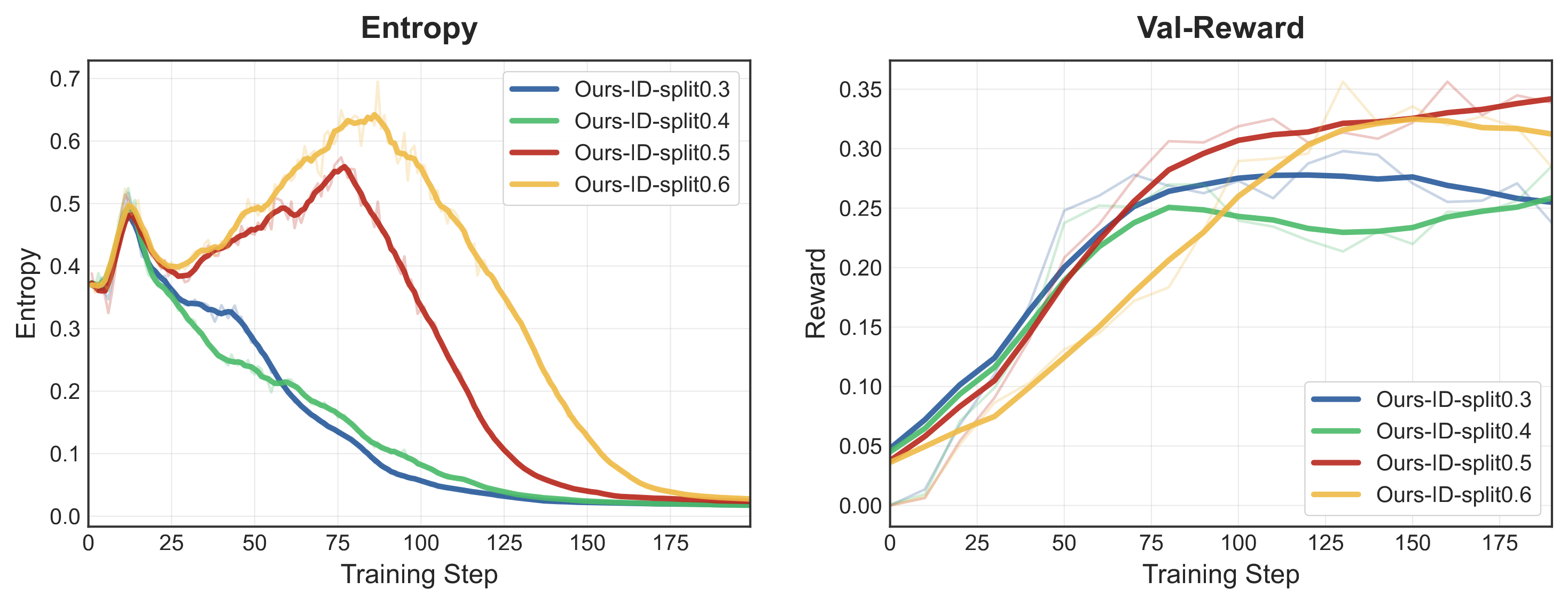
Figure 10: Entropy and validation score curves under different first-phase ratios (0.3, 0.4, 0.5, 0.6)

Results show that a balanced ratio of 0.5 achieves optimal performance:

• Too small (0.3/0.4): Entropy hasn’t reached a sufficient peak before declining
• Too large (0.6): The second phase converges too quickly, affecting final performance

---

7. Summary, Additional Analysis, and Outlook

This paper systematically studies the policy entropy control problem in RLVR from a gradient-preserving clipping perspective. Our main contributions include:

1. Theoretical insights: Precisely characterizing the mechanisms of four entropy-sensitive regions in the importance sampling ratio space
2. Regulation mechanism: Designing entropy regulation methods based on dynamic clipping thresholds that can independently control entropy increase and decrease
3. Control strategies: Proposing three entropy control strategies — ID, DID, and OD — that effectively mitigate entropy collapse and improve model performance

Additionally, further in-depth experimental analyses (clipping threshold correlations, token clipping probabilities, comparison with fixed-threshold methods) are available in our paper published on Arxiv. We validate the effectiveness and necessity of the dynamic clipping mechanism.

This work provides new theoretical tools and practical methods for understanding and controlling training dynamics in LLM reinforcement learning. In the future, we plan to explore more fine-grained adaptive entropy control mechanisms and extend this framework to broader RLVR application scenarios.

---

References

[1] Shen et al. “On Entropy Control in LLM-RL Algorithms.” 2025

[2] Schulman et al. “Proximal Policy Optimization Algorithms.” arXiv:1707.06347

[3] Yu et al. “DAPO: An Open-Source LLM Reinforcement Learning System at Scale.” arXiv:2503.14476

[4] Wang et al. “On the Entropy Dynamics in Reinforcement Fine-Tuning of Large Language Models”. arXiv:2602.03392

---

This article is based on our submitted work “Flexible Entropy Control in RLVR with Gradient-Preserving Perspective.” For questions or collaboration inquiries, please feel free to reach out.